一个非常非常简短的 diffusion model 学习,参考自 Lilian 的博客。
生成式模型概览
生成式模型通常都有着一个解构(压缩)至中间状态和重构(还原)的过程。
在使用训练好的模型生成数据的时候,我们可以从中间状态开始,然后还原得到我们想要的数据。
Diffusion
概览
Diffusion models are inspired by non-equilibrium thermodynamics.
They define a Markov chain of diffusion steps to slowly add random noise to data and then learn to reverse the diffusion process to construct desired data samples from the noise.
Unlike VAE or flow models, diffusion models are learned with a fixed procedure and the latent variable has high dimensionality (same as the original data).
不同于 GAN、VAE 等生成式模型,diffusion model 通过一个逐步加噪的过程来学习数据分布,再通过一个逐步去噪的过程来生成数据。
Forward diffusion process
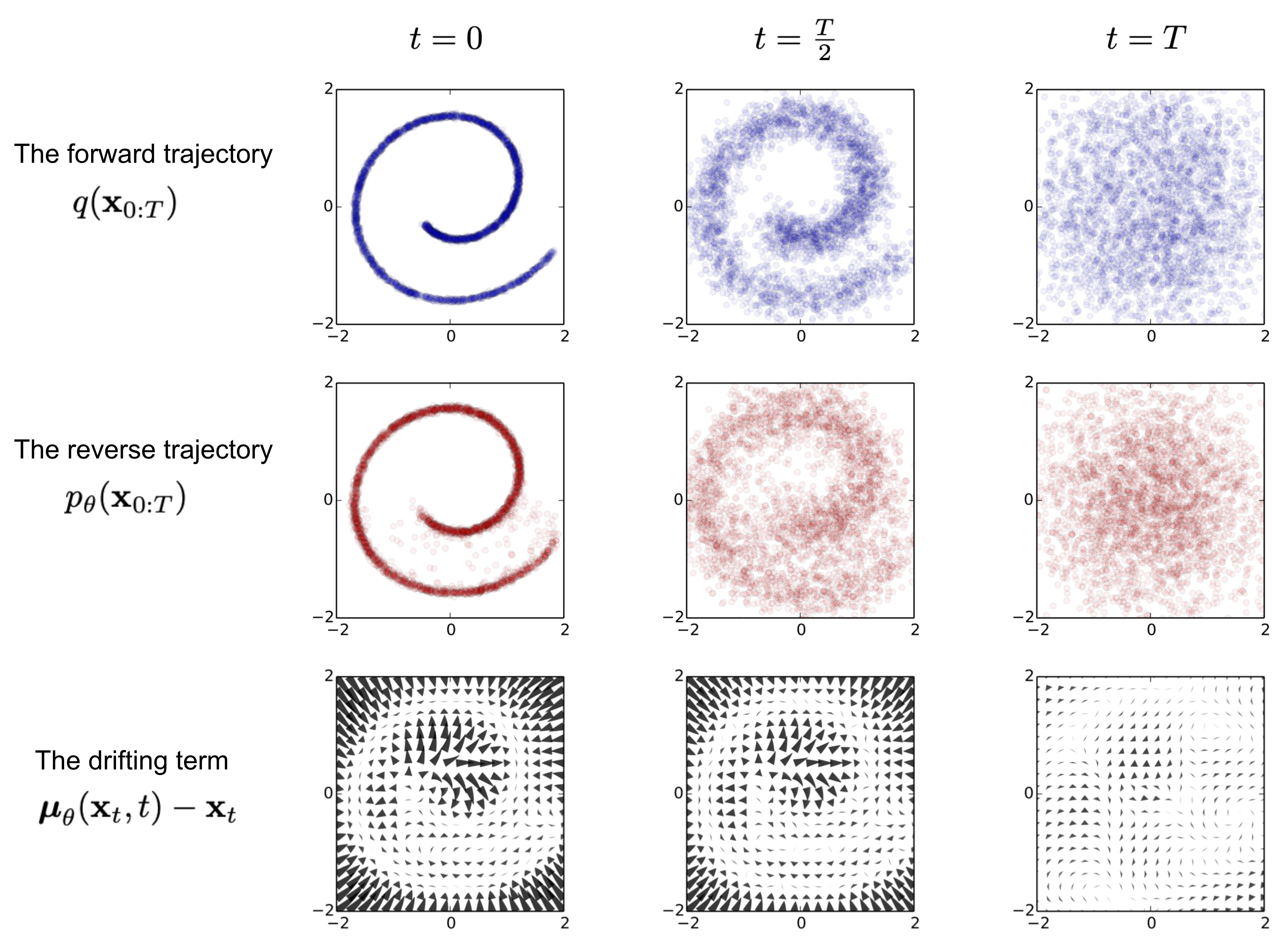
下图是 diffusion model 的一个示意图:
加噪声的过程可以写作:
q ( x t ∣ x t − 1 ) = N ( x t ; 1 − β t x t − 1 , β t I ) q ( x 1 : T ∣ x 0 ) = ∏ t = 1 T q ( x t ∣ x t − 1 ) q(\mathbf{x}_t \vert \mathbf{x}_{t-1}) = \mathcal{N}(\mathbf{x}_t; \sqrt{1 - \beta_t} \mathbf{x}_{t-1}, \beta_t\mathbf{I}) \quad \\
q(\mathbf{x}_{1:T} \vert \mathbf{x}_0) = \prod^T_{t=1} q(\mathbf{x}_t \vert \mathbf{x}_{t-1})
q ( x t ∣ x t − 1 ) = N ( x t ; 1 − β t x t − 1 , β t I ) q ( x 1 : T ∣ x 0 ) = t = 1 ∏ T q ( x t ∣ x t − 1 )
这个可以通过一个高斯采样来实现,其中 β t \beta_t β t α t = 1 − β t , α ˉ t = ∏ i = 1 t α i \alpha_t = 1 - \beta_t, \bar{\alpha}_t = \prod_{i=1}^t \alpha_i α t = 1 − β t , α ˉ t = ∏ i = 1 t α i
x t = α t x t − 1 + 1 − α t ϵ t − 1 ;where ϵ t − 1 , ϵ t − 2 , ⋯ ∼ N ( 0 , I ) = α t α t − 1 x t − 2 + 1 − α t α t − 1 ϵ ˉ t − 2 ;where ϵ ˉ t − 2 merges two Gaussians. = … = α ˉ t x 0 + 1 − α ˉ t ϵ q ( x t ∣ x 0 ) = N ( x t ; α ˉ t x 0 , ( 1 − α ˉ t ) I ) \begin{aligned}
\mathbf{x}_t
&= \sqrt{\alpha_t}\mathbf{x}_{t-1} + \sqrt{1 - \alpha_t}\boldsymbol{\epsilon}_{t-1} & \text{ ;where } \boldsymbol{\epsilon}_{t-1}, \boldsymbol{\epsilon}_{t-2}, \dots \sim \mathcal{N}(\mathbf{0}, \mathbf{I}) \\
&= \sqrt{\alpha_t \alpha_{t-1}} \mathbf{x}_{t-2} + \sqrt{1 - \alpha_t \alpha_{t-1}} \bar{\boldsymbol{\epsilon}}_{t-2} & \text{ ;where } \bar{\boldsymbol{\epsilon}}_{t-2} \text{ merges two Gaussians.} \\
&= \dots \\
&= \sqrt{\bar{\alpha}_t}\mathbf{x}_0 + \sqrt{1 - \bar{\alpha}_t}\boldsymbol{\epsilon} \\
q(\mathbf{x}_t \vert \mathbf{x}_0) &= \mathcal{N}(\mathbf{x}_t; \sqrt{\bar{\alpha}_t} \mathbf{x}_0, (1 - \bar{\alpha}_t)\mathbf{I})
\end{aligned}
x t q ( x t ∣ x 0 ) = α t x t − 1 + 1 − α t ϵ t − 1 = α t α t − 1 x t − 2 + 1 − α t α t − 1 ϵ ˉ t − 2 = … = α ˉ t x 0 + 1 − α ˉ t ϵ = N ( x t ; α ˉ t x 0 , ( 1 − α ˉ t ) I ) ;where ϵ t − 1 , ϵ t − 2 , ⋯ ∼ N ( 0 , I ) ;where ϵ ˉ t − 2 merges two Gaussians.
ϵ \boldsymbol{\epsilon} ϵ β 1 < β 2 < ⋯ < β T \beta_1 < \beta_2 < \dots < \beta_T β 1 < β 2 < ⋯ < β T α ˉ 1 > ⋯ > α ˉ T \bar{\alpha}_1 > \dots > \bar{\alpha}_T α ˉ 1 > ⋯ > α ˉ T
Reverse diffusion process
如果我们可以逆转上述 q ( x t ∣ x t − 1 ) q(\mathbf{x}_t \vert \mathbf{x}_{t-1}) q ( x t ∣ x t − 1 ) q ( x t − 1 ∣ x t ) q(\mathbf{x}_{t-1} \vert \mathbf{x}_t) q ( x t − 1 ∣ x t ) x T ∼ N ( 0 , I ) \mathbf{x}_T \sim \mathcal{N}(\mathbf{0}, \mathbf{I}) x T ∼ N ( 0 , I ) x 0 \mathbf{x}_0 x 0 β t \beta_t β t q ( x t ∣ x t − 1 ) q(\mathbf{x}_t \vert \mathbf{x}_{t-1}) q ( x t ∣ x t − 1 ) p θ p_\theta p θ
p θ ( x 0 : T ) = p ( x T ) ∏ t = 1 T p θ ( x t − 1 ∣ x t ) p θ ( x t − 1 ∣ x t ) = N ( x t − 1 ; μ θ ( x t , t ) , Σ θ ( x t , t ) ) p_\theta(\mathbf{x}_{0:T}) = p(\mathbf{x}_T) \prod^T_{t=1} p_\theta(\mathbf{x}_{t-1} \vert \mathbf{x}_t) \quad \\
p_\theta(\mathbf{x}_{t-1} \vert \mathbf{x}_t) = \mathcal{N}(\mathbf{x}_{t-1}; \boldsymbol{\mu}_\theta(\mathbf{x}_t, t), \boldsymbol{\Sigma}_\theta(\mathbf{x}_t, t))
p θ ( x 0 : T ) = p ( x T ) t = 1 ∏ T p θ ( x t − 1 ∣ x t ) p θ ( x t − 1 ∣ x t ) = N ( x t − 1 ; μ θ ( x t , t ) , Σ θ ( x t , t ))
值得注意的是,这个逆条件概率在基于 x 0 \mathbf{x}_0 x 0
q ( x t − 1 ∣ x t , x 0 ) = N ( x t − 1 ; μ ~ ( x t , x 0 ) , β ~ t I ) q(\mathbf{x}_{t-1} \vert \mathbf{x}_t, \mathbf{x}_0) = \mathcal{N}(\mathbf{x}_{t-1}; \color{blue}{\tilde{\boldsymbol{\mu}}}(\mathbf{x}_t, \mathbf{x}_0), \color{red}{\tilde{\beta}_t} \mathbf{I})
q ( x t − 1 ∣ x t , x 0 ) = N ( x t − 1 ; μ ~ ( x t , x 0 ) , β ~ t I )
通过贝叶斯法则可得:
q ( x t − 1 ∣ x t , x 0 ) = q ( x t ∣ x t − 1 , x 0 ) q ( x t − 1 ∣ x 0 ) q ( x t ∣ x 0 ) ∝ exp ( − 1 2 ( ( x t − α t x t − 1 ) 2 β t + ( x t − 1 − α ˉ t − 1 x 0 ) 2 1 − α ˉ t − 1 − ( x t − α ˉ t x 0 ) 2 1 − α ˉ t ) ) = exp ( − 1 2 ( x t 2 − 2 α t x t x t − 1 + α t x t − 1 2 β t + x t − 1 2 − 2 α ˉ t − 1 x 0 x t − 1 + α ˉ t − 1 x 0 2 1 − α ˉ t − 1 − ( x t − α ˉ t x 0 ) 2 1 − α ˉ t ) ) = exp ( − 1 2 ( ( α t β t + 1 1 − α ˉ t − 1 ) x t − 1 2 − ( 2 α t β t x t + 2 α ˉ t − 1 1 − α ˉ t − 1 x 0 ) x t − 1 + C ( x t , x 0 ) ) ) \begin{aligned}
q(\mathbf{x}_{t-1} \vert \mathbf{x}_t, \mathbf{x}_0)
&= q(\mathbf{x}_t \vert \mathbf{x}_{t-1}, \mathbf{x}_0) \frac{ q(\mathbf{x}_{t-1} \vert \mathbf{x}_0) }{ q(\mathbf{x}_t \vert \mathbf{x}_0) } \\
&\propto \exp \Big(-\frac{1}{2} \big(\frac{(\mathbf{x}_t - \sqrt{\alpha_t} \mathbf{x}_{t-1})^2}{\beta_t} + \frac{(\mathbf{x}_{t-1} - \sqrt{\bar{\alpha}_{t-1}} \mathbf{x}_0)^2}{1-\bar{\alpha}_{t-1}} - \frac{(\mathbf{x}_t - \sqrt{\bar{\alpha}_t} \mathbf{x}_0)^2}{1-\bar{\alpha}_t} \big) \Big) \\
&= \exp \Big(-\frac{1}{2} \big(\frac{\mathbf{x}_t^2 - 2\sqrt{\alpha_t} \mathbf{x}_t \color{blue}{\mathbf{x}_{t-1}} \color{black}{+ \alpha_t} \color{red}{\mathbf{x}_{t-1}^2} }{\beta_t} + \frac{ \color{red}{\mathbf{x}_{t-1}^2} \color{black}{- 2 \sqrt{\bar{\alpha}_{t-1}} \mathbf{x}_0} \color{blue}{\mathbf{x}_{t-1}} \color{black}{+ \bar{\alpha}_{t-1} \mathbf{x}_0^2} }{1-\bar{\alpha}_{t-1}} - \frac{(\mathbf{x}_t - \sqrt{\bar{\alpha}_t} \mathbf{x}_0)^2}{1-\bar{\alpha}_t} \big) \Big) \\
&= \exp\Big( -\frac{1}{2} \big( \color{red}{(\frac{\alpha_t}{\beta_t} + \frac{1}{1 - \bar{\alpha}_{t-1}})} \mathbf{x}_{t-1}^2 - \color{blue}{(\frac{2\sqrt{\alpha_t}}{\beta_t} \mathbf{x}_t + \frac{2\sqrt{\bar{\alpha}_{t-1}}}{1 - \bar{\alpha}_{t-1}} \mathbf{x}_0)} \mathbf{x}_{t-1} \color{black}{ + C(\mathbf{x}_t, \mathbf{x}_0) \big) \Big)}
\end{aligned}
q ( x t − 1 ∣ x t , x 0 ) = q ( x t ∣ x t − 1 , x 0 ) q ( x t ∣ x 0 ) q ( x t − 1 ∣ x 0 ) ∝ exp ( − 2 1 ( β t ( x t − α t x t − 1 ) 2 + 1 − α ˉ t − 1 ( x t − 1 − α ˉ t − 1 x 0 ) 2 − 1 − α ˉ t ( x t − α ˉ t x 0 ) 2 ) ) = exp ( − 2 1 ( β t x t 2 − 2 α t x t x t − 1 + α t x t − 1 2 + 1 − α ˉ t − 1 x t − 1 2 − 2 α ˉ t − 1 x 0 x t − 1 + α ˉ t − 1 x 0 2 − 1 − α ˉ t ( x t − α ˉ t x 0 ) 2 ) ) = exp ( − 2 1 ( ( β t α t + 1 − α ˉ t − 1 1 ) x t − 1 2 − ( β t 2 α t x t + 1 − α ˉ t − 1 2 α ˉ t − 1 x 0 ) x t − 1 + C ( x t , x 0 ) ) )
第二行的正比由高斯函数的公式得到,即 f ( x ) = 1 σ 2 π e − ( x − μ ) 2 2 σ 2 {\displaystyle f(x)={\frac {1}{\sigma {\sqrt {2\pi }}}}\;e^{-{\frac {\left(x-\mu \right)^{2}}{2\sigma ^{2}}}}\!} f ( x ) = σ 2 π 1 e − 2 σ 2 ( x − μ ) 2
β ~ t = 1 / ( α t β t + 1 1 − α ˉ t − 1 ) = 1 / ( α t − α ˉ t + β t β t ( 1 − α ˉ t − 1 ) ) = 1 − α ˉ t − 1 1 − α ˉ t ⋅ β t μ ~ t ( x t , x 0 ) = ( α t β t x t + α ˉ t − 1 1 − α ˉ t − 1 x 0 ) / ( α t β t + 1 1 − α ˉ t − 1 ) = ( α t β t x t + α ˉ t − 1 1 − α ˉ t − 1 x 0 ) 1 − α ˉ t − 1 1 − α ˉ t ⋅ β t = α t ( 1 − α ˉ t − 1 ) 1 − α ˉ t x t + α ˉ t − 1 β t 1 − α ˉ t x 0 \begin{aligned}
\tilde{\beta}_t
&= 1/(\frac{\alpha_t}{\beta_t} + \frac{1}{1 - \bar{\alpha}_{t-1}})
= 1/(\frac{\alpha_t - \bar{\alpha}_t + \beta_t}{\beta_t(1 - \bar{\alpha}_{t-1})})
= \color{green}{\frac{1 - \bar{\alpha}_{t-1}}{1 - \bar{\alpha}_t} \cdot \beta_t} \\
\tilde{\boldsymbol{\mu}}_t (\mathbf{x}_t, \mathbf{x}_0)
&= (\frac{\sqrt{\alpha_t}}{\beta_t} \mathbf{x}_t + \frac{\sqrt{\bar{\alpha}_{t-1} }}{1 - \bar{\alpha}_{t-1}} \mathbf{x}_0)/(\frac{\alpha_t}{\beta_t} + \frac{1}{1 - \bar{\alpha}_{t-1}}) \\
&= (\frac{\sqrt{\alpha_t}}{\beta_t} \mathbf{x}_t + \frac{\sqrt{\bar{\alpha}_{t-1} }}{1 - \bar{\alpha}_{t-1}} \mathbf{x}_0) \color{green}{\frac{1 - \bar{\alpha}_{t-1}}{1 - \bar{\alpha}_t} \cdot \beta_t} \\
&= \frac{\sqrt{\alpha_t}(1 - \bar{\alpha}_{t-1})}{1 - \bar{\alpha}_t} \mathbf{x}_t + \frac{\sqrt{\bar{\alpha}_{t-1}}\beta_t}{1 - \bar{\alpha}_t} \mathbf{x}_0\\
\end{aligned}
β ~ t μ ~ t ( x t , x 0 ) = 1/ ( β t α t + 1 − α ˉ t − 1 1 ) = 1/ ( β t ( 1 − α ˉ t − 1 ) α t − α ˉ t + β t ) = 1 − α ˉ t 1 − α ˉ t − 1 ⋅ β t = ( β t α t x t + 1 − α ˉ t − 1 α ˉ t − 1 x 0 ) / ( β t α t + 1 − α ˉ t − 1 1 ) = ( β t α t x t + 1 − α ˉ t − 1 α ˉ t − 1 x 0 ) 1 − α ˉ t 1 − α ˉ t − 1 ⋅ β t = 1 − α ˉ t α t ( 1 − α ˉ t − 1 ) x t + 1 − α ˉ t α ˉ t − 1 β t x 0
进一步考虑到之前的推导 x 0 = 1 α ˉ t ( x t − 1 − α ˉ t ϵ t ) \mathbf{x}_0 = \frac{1}{\sqrt{\bar{\alpha}_t}}(\mathbf{x}_t - \sqrt{1 - \bar{\alpha}_t}\boldsymbol{\epsilon}_t) x 0 = α ˉ t 1 ( x t − 1 − α ˉ t ϵ t )
μ ~ t = α t ( 1 − α ˉ t − 1 ) 1 − α ˉ t x t + α ˉ t − 1 β t 1 − α ˉ t 1 α ˉ t ( x t − 1 − α ˉ t ϵ t ) = 1 α t ( x t − 1 − α t 1 − α ˉ t ϵ t ) \begin{aligned}
\tilde{\boldsymbol{\mu}}_t
&= \frac{\sqrt{\alpha_t}(1 - \bar{\alpha}_{t-1})}{1 - \bar{\alpha}_t} \mathbf{x}_t + \frac{\sqrt{\bar{\alpha}_{t-1}}\beta_t}{1 - \bar{\alpha}_t} \frac{1}{\sqrt{\bar{\alpha}_t}}(\mathbf{x}_t - \sqrt{1 - \bar{\alpha}_t}\boldsymbol{\epsilon}_t) \\
&= \color{cyan}{\frac{1}{\sqrt{\alpha_t}} \Big( \mathbf{x}_t - \frac{1 - \alpha_t}{\sqrt{1 - \bar{\alpha}_t}} \boldsymbol{\epsilon}_t \Big)}
\end{aligned}
μ ~ t = 1 − α ˉ t α t ( 1 − α ˉ t − 1 ) x t + 1 − α ˉ t α ˉ t − 1 β t α ˉ t 1 ( x t − 1 − α ˉ t ϵ t ) = α t 1 ( x t − 1 − α ˉ t 1 − α t ϵ t )
Parameterization
上述逆过程 p θ ( x t − 1 ∣ x t ) = N ( x t − 1 ; μ θ ( x t , t ) , Σ θ ( x t , t ) ) ) p_\theta(\mathbf{x}_{t-1} \vert \mathbf{x}_t) = \mathcal{N}(\mathbf{x}_{t-1}; \boldsymbol{\mu}_\theta(\mathbf{x}_t, t), \boldsymbol{\Sigma}_\theta(\mathbf{x}_t, t))) p θ ( x t − 1 ∣ x t ) = N ( x t − 1 ; μ θ ( x t , t ) , Σ θ ( x t , t ))) μ θ \boldsymbol{\mu}_\theta μ θ μ ~ t = 1 α t ( x t − 1 − α t 1 − α ˉ t ϵ t ) \tilde{\boldsymbol{\mu}}_t = \frac{1}{\sqrt{\alpha_t}} \Big( \mathbf{x}_t - \frac{1 - \alpha_t}{\sqrt{1 - \bar{\alpha}_t}} \boldsymbol{\epsilon}_t \Big) μ ~ t = α t 1 ( x t − 1 − α ˉ t 1 − α t ϵ t ) x t \mathbf{x}_t x t ϵ t \boldsymbol{\epsilon}_t ϵ t t t t
μ θ ( x t , t ) = 1 α t ( x t − 1 − α t 1 − α ˉ t ϵ θ ( x t , t ) ) Thus x t − 1 = N ( x t − 1 ; 1 α t ( x t − 1 − α t 1 − α ˉ t ϵ θ ( x t , t ) ) , Σ θ ( x t , t ) ) \begin{aligned}
\boldsymbol{\mu}_\theta(\mathbf{x}_t, t) &= \color{cyan}{\frac{1}{\sqrt{\alpha_t}} \Big( \mathbf{x}_t - \frac{1 - \alpha_t}{\sqrt{1 - \bar{\alpha}_t}} \boldsymbol{\epsilon}_\theta(\mathbf{x}_t, t) \Big)} \\
\text{Thus }\mathbf{x}_{t-1} &= \mathcal{N}(\mathbf{x}_{t-1}; \frac{1}{\sqrt{\alpha_t}} \Big( \mathbf{x}_t - \frac{1 - \alpha_t}{\sqrt{1 - \bar{\alpha}_t}} \boldsymbol{\epsilon}_\theta(\mathbf{x}_t, t) \Big), \boldsymbol{\Sigma}_\theta(\mathbf{x}_t, t))
\end{aligned}
μ θ ( x t , t ) Thus x t − 1 = α t 1 ( x t − 1 − α ˉ t 1 − α t ϵ θ ( x t , t ) ) = N ( x t − 1 ; α t 1 ( x t − 1 − α ˉ t 1 − α t ϵ θ ( x t , t ) ) , Σ θ ( x t , t ))
Loss Function
Training is performed by optimizing the usual variational lower bound (VLB) on negative log likelihood:
L CE = − E q ( x 0 ) log p θ ( x 0 ) = − E q ( x 0 ) log ( ∫ p θ ( x 0 : T ) d x 1 : T ) = − E q ( x 0 ) log ( ∫ q ( x 1 : T ∣ x 0 ) p θ ( x 0 : T ) q ( x 1 : T ∣ x 0 ) d x 1 : T ) = − E q ( x 0 ) log ( E q ( x 1 : T ∣ x 0 ) p θ ( x 0 : T ) q ( x 1 : T ∣ x 0 ) ) ≤ − E q ( x 0 : T ) log p θ ( x 0 : T ) q ( x 1 : T ∣ x 0 ) = E q ( x 0 : T ) [ log q ( x 1 : T ∣ x 0 ) p θ ( x 0 : T ) ] = L VLB \begin{aligned}
L_\text{CE}
&= - \mathbb{E}_{q(\mathbf{x}_0)} \log p_\theta(\mathbf{x}_0) \\
&= - \mathbb{E}_{q(\mathbf{x}_0)} \log \Big( \int p_\theta(\mathbf{x}_{0:T}) d\mathbf{x}_{1:T} \Big) \\
&= - \mathbb{E}_{q(\mathbf{x}_0)} \log \Big( \int q(\mathbf{x}_{1:T} \vert \mathbf{x}_0) \frac{p_\theta(\mathbf{x}_{0:T})}{q(\mathbf{x}_{1:T} \vert \mathbf{x}_{0})} d\mathbf{x}_{1:T} \Big) \\
&= - \mathbb{E}_{q(\mathbf{x}_0)} \log \Big( \mathbb{E}_{q(\mathbf{x}_{1:T} \vert \mathbf{x}_0)} \frac{p_\theta(\mathbf{x}_{0:T})}{q(\mathbf{x}_{1:T} \vert \mathbf{x}_{0})} \Big) \\
&\leq - \mathbb{E}_{q(\mathbf{x}_{0:T})} \log \frac{p_\theta(\mathbf{x}_{0:T})}{q(\mathbf{x}_{1:T} \vert \mathbf{x}_{0})} \\
&= \mathbb{E}_{q(\mathbf{x}_{0:T})}\Big[\log \frac{q(\mathbf{x}_{1:T} \vert \mathbf{x}_{0})}{p_\theta(\mathbf{x}_{0:T})} \Big] = L_\text{VLB}
\end{aligned}
L CE = − E q ( x 0 ) log p θ ( x 0 ) = − E q ( x 0 ) log ( ∫ p θ ( x 0 : T ) d x 1 : T ) = − E q ( x 0 ) log ( ∫ q ( x 1 : T ∣ x 0 ) q ( x 1 : T ∣ x 0 ) p θ ( x 0 : T ) d x 1 : T ) = − E q ( x 0 ) log ( E q ( x 1 : T ∣ x 0 ) q ( x 1 : T ∣ x 0 ) p θ ( x 0 : T ) ) ≤ − E q ( x 0 : T ) log q ( x 1 : T ∣ x 0 ) p θ ( x 0 : T ) = E q ( x 0 : T ) [ log p θ ( x 0 : T ) q ( x 1 : T ∣ x 0 ) ] = L VLB
L VLB = E q ( x 0 : T ) [ log q ( x 1 : T ∣ x 0 ) p θ ( x 0 : T ) ] = E q [ log ∏ t = 1 T q ( x t ∣ x t − 1 ) p θ ( x T ) ∏ t = 1 T p θ ( x t − 1 ∣ x t ) ] = E q [ − log p θ ( x T ) + ∑ t = 1 T log q ( x t ∣ x t − 1 ) p θ ( x t − 1 ∣ x t ) ] = E q [ − log p θ ( x T ) + ∑ t = 2 T log q ( x t ∣ x t − 1 ) p θ ( x t − 1 ∣ x t ) + log q ( x 1 ∣ x 0 ) p θ ( x 0 ∣ x 1 ) ] = E q [ − log p θ ( x T ) + ∑ t = 2 T log ( q ( x t − 1 ∣ x t , x 0 ) p θ ( x t − 1 ∣ x t ) ⋅ q ( x t ∣ x 0 ) q ( x t − 1 ∣ x 0 ) ) + log q ( x 1 ∣ x 0 ) p θ ( x 0 ∣ x 1 ) ] = E q [ − log p θ ( x T ) + ∑ t = 2 T log q ( x t − 1 ∣ x t , x 0 ) p θ ( x t − 1 ∣ x t ) + ∑ t = 2 T log q ( x t ∣ x 0 ) q ( x t − 1 ∣ x 0 ) + log q ( x 1 ∣ x 0 ) p θ ( x 0 ∣ x 1 ) ] = E q [ − log p θ ( x T ) + ∑ t = 2 T log q ( x t − 1 ∣ x t , x 0 ) p θ ( x t − 1 ∣ x t ) + log q ( x T ∣ x 0 ) q ( x 1 ∣ x 0 ) + log q ( x 1 ∣ x 0 ) p θ ( x 0 ∣ x 1 ) ] = E q [ log q ( x T ∣ x 0 ) p θ ( x T ) + ∑ t = 2 T log q ( x t − 1 ∣ x t , x 0 ) p θ ( x t − 1 ∣ x t ) − log p θ ( x 0 ∣ x 1 ) ] = E q [ D KL ( q ( x T ∣ x 0 ) ∥ p θ ( x T ) ) ⏟ L T + ∑ t = 2 T D KL ( q ( x t − 1 ∣ x t , x 0 ) ∥ p θ ( x t − 1 ∣ x t ) ) ⏟ L t − 1 − log p θ ( x 0 ∣ x 1 ) ⏟ L 0 ] \begin{aligned}
L_\text{VLB}
&= \mathbb{E}_{q(\mathbf{x}_{0:T})} \Big[ \log\frac{q(\mathbf{x}_{1:T}\vert\mathbf{x}_0)}{p_\theta(\mathbf{x}_{0:T})} \Big] \\
&= \mathbb{E}_q \Big[ \log\frac{\prod_{t=1}^T q(\mathbf{x}_t\vert\mathbf{x}_{t-1})}{ p_\theta(\mathbf{x}_T) \prod_{t=1}^T p_\theta(\mathbf{x}_{t-1} \vert\mathbf{x}_t) } \Big] \\
&= \mathbb{E}_q \Big[ -\log p_\theta(\mathbf{x}_T) + \sum_{t=1}^T \log \frac{q(\mathbf{x}_t\vert\mathbf{x}_{t-1})}{p_\theta(\mathbf{x}_{t-1} \vert\mathbf{x}_t)} \Big] \\
&= \mathbb{E}_q \Big[ -\log p_\theta(\mathbf{x}_T) + \sum_{t=2}^T \log \frac{q(\mathbf{x}_t\vert\mathbf{x}_{t-1})}{p_\theta(\mathbf{x}_{t-1} \vert\mathbf{x}_t)} + \log\frac{q(\mathbf{x}_1 \vert \mathbf{x}_0)}{p_\theta(\mathbf{x}_0 \vert \mathbf{x}_1)} \Big] \\
&= \mathbb{E}_q \Big[ -\log p_\theta(\mathbf{x}_T) + \sum_{t=2}^T \log \Big( \frac{q(\mathbf{x}_{t-1} \vert \mathbf{x}_t, \mathbf{x}_0)}{p_\theta(\mathbf{x}_{t-1} \vert\mathbf{x}_t)}\cdot \frac{q(\mathbf{x}_t \vert \mathbf{x}_0)}{q(\mathbf{x}_{t-1}\vert\mathbf{x}_0)} \Big) + \log \frac{q(\mathbf{x}_1 \vert \mathbf{x}_0)}{p_\theta(\mathbf{x}_0 \vert \mathbf{x}_1)} \Big] \\
&= \mathbb{E}_q \Big[ -\log p_\theta(\mathbf{x}_T) + \sum_{t=2}^T \log \frac{q(\mathbf{x}_{t-1} \vert \mathbf{x}_t, \mathbf{x}_0)}{p_\theta(\mathbf{x}_{t-1} \vert\mathbf{x}_t)} + \sum_{t=2}^T \log \frac{q(\mathbf{x}_t \vert \mathbf{x}_0)}{q(\mathbf{x}_{t-1} \vert \mathbf{x}_0)} + \log\frac{q(\mathbf{x}_1 \vert \mathbf{x}_0)}{p_\theta(\mathbf{x}_0 \vert \mathbf{x}_1)} \Big] \\
&= \mathbb{E}_q \Big[ -\log p_\theta(\mathbf{x}_T) + \sum_{t=2}^T \log \frac{q(\mathbf{x}_{t-1} \vert \mathbf{x}_t, \mathbf{x}_0)}{p_\theta(\mathbf{x}_{t-1} \vert\mathbf{x}_t)} + \log\frac{q(\mathbf{x}_T \vert \mathbf{x}_0)}{q(\mathbf{x}_1 \vert \mathbf{x}_0)} + \log \frac{q(\mathbf{x}_1 \vert \mathbf{x}_0)}{p_\theta(\mathbf{x}_0 \vert \mathbf{x}_1)} \Big]\\
&= \mathbb{E}_q \Big[ \log\frac{q(\mathbf{x}_T \vert \mathbf{x}_0)}{p_\theta(\mathbf{x}_T)} + \sum_{t=2}^T \log \frac{q(\mathbf{x}_{t-1} \vert \mathbf{x}_t, \mathbf{x}_0)}{p_\theta(\mathbf{x}_{t-1} \vert\mathbf{x}_t)} - \log p_\theta(\mathbf{x}_0 \vert \mathbf{x}_1) \Big] \\
&= \mathbb{E}_q [\underbrace{D_\text{KL}(q(\mathbf{x}_T \vert \mathbf{x}_0) \parallel p_\theta(\mathbf{x}_T))}_{L_T} + \sum_{t=2}^T \underbrace{D_\text{KL}(q(\mathbf{x}_{t-1} \vert \mathbf{x}_t, \mathbf{x}_0) \parallel p_\theta(\mathbf{x}_{t-1} \vert\mathbf{x}_t))}_{L_{t-1}} \underbrace{- \log p_\theta(\mathbf{x}_0 \vert \mathbf{x}_1)}_{L_0} ]
\end{aligned}
L VLB = E q ( x 0 : T ) [ log p θ ( x 0 : T ) q ( x 1 : T ∣ x 0 ) ] = E q [ log p θ ( x T ) ∏ t = 1 T p θ ( x t − 1 ∣ x t ) ∏ t = 1 T q ( x t ∣ x t − 1 ) ] = E q [ − log p θ ( x T ) + t = 1 ∑ T log p θ ( x t − 1 ∣ x t ) q ( x t ∣ x t − 1 ) ] = E q [ − log p θ ( x T ) + t = 2 ∑ T log p θ ( x t − 1 ∣ x t ) q ( x t ∣ x t − 1 ) + log p θ ( x 0 ∣ x 1 ) q ( x 1 ∣ x 0 ) ] = E q [ − log p θ ( x T ) + t = 2 ∑ T log ( p θ ( x t − 1 ∣ x t ) q ( x t − 1 ∣ x t , x 0 ) ⋅ q ( x t − 1 ∣ x 0 ) q ( x t ∣ x 0 ) ) + log p θ ( x 0 ∣ x 1 ) q ( x 1 ∣ x 0 ) ] = E q [ − log p θ ( x T ) + t = 2 ∑ T log p θ ( x t − 1 ∣ x t ) q ( x t − 1 ∣ x t , x 0 ) + t = 2 ∑ T log q ( x t − 1 ∣ x 0 ) q ( x t ∣ x 0 ) + log p θ ( x 0 ∣ x 1 ) q ( x 1 ∣ x 0 ) ] = E q [ − log p θ ( x T ) + t = 2 ∑ T log p θ ( x t − 1 ∣ x t ) q ( x t − 1 ∣ x t , x 0 ) + log q ( x 1 ∣ x 0 ) q ( x T ∣ x 0 ) + log p θ ( x 0 ∣ x 1 ) q ( x 1 ∣ x 0 ) ] = E q [ log p θ ( x T ) q ( x T ∣ x 0 ) + t = 2 ∑ T log p θ ( x t − 1 ∣ x t ) q ( x t − 1 ∣ x t , x 0 ) − log p θ ( x 0 ∣ x 1 ) ] = E q [ L T D KL ( q ( x T ∣ x 0 ) ∥ p θ ( x T )) + t = 2 ∑ T L t − 1 D KL ( q ( x t − 1 ∣ x t , x 0 ) ∥ p θ ( x t − 1 ∣ x t )) L 0 − log p θ ( x 0 ∣ x 1 ) ]
所以在 t t t μ ~ \tilde{\boldsymbol{\mu}} μ ~
L t = E x 0 , ϵ [ 1 2 ∥ Σ θ ( x t , t ) ∥ 2 2 ∥ μ ~ t ( x t , x 0 ) − μ θ ( x t , t ) ∥ 2 ] = E x 0 , ϵ [ 1 2 ∥ Σ θ ∥ 2 2 ∥ 1 α t ( x t − 1 − α t 1 − α ˉ t ϵ t ) − 1 α t ( x t − 1 − α t 1 − α ˉ t ϵ θ ( x t , t ) ) ∥ 2 ] = E x 0 , ϵ [ ( 1 − α t ) 2 2 α t ( 1 − α ˉ t ) ∥ Σ θ ∥ 2 2 ∥ ϵ t − ϵ θ ( x t , t ) ∥ 2 ] = E x 0 , ϵ [ ( 1 − α t ) 2 2 α t ( 1 − α ˉ t ) ∥ Σ θ ∥ 2 2 ∥ ϵ t − ϵ θ ( α ˉ t x 0 + 1 − α ˉ t ϵ t , t ) ∥ 2 ] \begin{aligned}
L_t
&= \mathbb{E}_{\mathbf{x}_0, \boldsymbol{\epsilon}} \Big[\frac{1}{2 \| \boldsymbol{\Sigma}_\theta(\mathbf{x}_t, t) \|^2_2} \| \color{blue}{\tilde{\boldsymbol{\mu}}_t(\mathbf{x}_t, \mathbf{x}_0)} - \color{green}{\boldsymbol{\mu}_\theta(\mathbf{x}_t, t)} \|^2 \Big] \\
&= \mathbb{E}_{\mathbf{x}_0, \boldsymbol{\epsilon}} \Big[\frac{1}{2 \|\boldsymbol{\Sigma}_\theta \|^2_2} \| \color{blue}{\frac{1}{\sqrt{\alpha_t}} \Big( \mathbf{x}_t - \frac{1 - \alpha_t}{\sqrt{1 - \bar{\alpha}_t}} \boldsymbol{\epsilon}_t \Big)} - \color{green}{\frac{1}{\sqrt{\alpha_t}} \Big( \mathbf{x}_t - \frac{1 - \alpha_t}{\sqrt{1 - \bar{\alpha}_t}} \boldsymbol{\boldsymbol{\epsilon}}_\theta(\mathbf{x}_t, t) \Big)} \|^2 \Big] \\
&= \mathbb{E}_{\mathbf{x}_0, \boldsymbol{\epsilon}} \Big[\frac{ (1 - \alpha_t)^2 }{2 \alpha_t (1 - \bar{\alpha}_t) \| \boldsymbol{\Sigma}_\theta \|^2_2} \|\boldsymbol{\epsilon}_t - \boldsymbol{\epsilon}_\theta(\mathbf{x}_t, t)\|^2 \Big] \\
&= \mathbb{E}_{\mathbf{x}_0, \boldsymbol{\epsilon}} \Big[\frac{ (1 - \alpha_t)^2 }{2 \alpha_t (1 - \bar{\alpha}_t) \| \boldsymbol{\Sigma}_\theta \|^2_2} \|\boldsymbol{\epsilon}_t - \boldsymbol{\epsilon}_\theta(\sqrt{\bar{\alpha}_t}\mathbf{x}_0 + \sqrt{1 - \bar{\alpha}_t}\boldsymbol{\epsilon}_t, t)\|^2 \Big]
\end{aligned}
L t = E x 0 , ϵ [ 2∥ Σ θ ( x t , t ) ∥ 2 2 1 ∥ μ ~ t ( x t , x 0 ) − μ θ ( x t , t ) ∥ 2 ] = E x 0 , ϵ [ 2∥ Σ θ ∥ 2 2 1 ∥ α t 1 ( x t − 1 − α ˉ t 1 − α t ϵ t ) − α t 1 ( x t − 1 − α ˉ t 1 − α t ϵ θ ( x t , t ) ) ∥ 2 ] = E x 0 , ϵ [ 2 α t ( 1 − α ˉ t ) ∥ Σ θ ∥ 2 2 ( 1 − α t ) 2 ∥ ϵ t − ϵ θ ( x t , t ) ∥ 2 ] = E x 0 , ϵ [ 2 α t ( 1 − α ˉ t ) ∥ Σ θ ∥ 2 2 ( 1 − α t ) 2 ∥ ϵ t − ϵ θ ( α ˉ t x 0 + 1 − α ˉ t ϵ t , t ) ∥ 2 ]
忽略权重项进行简化可得:
L t simple = E t ∼ [ 1 , T ] , x 0 , ϵ t [ ∥ ϵ t − ϵ θ ( x t , t ) ∥ 2 ] = E t ∼ [ 1 , T ] , x 0 , ϵ t [ ∥ ϵ t − ϵ θ ( α ˉ t x 0 + 1 − α ˉ t ϵ t , t ) ∥ 2 ] \begin{aligned}
L_t^\text{simple}
&= \mathbb{E}_{t \sim [1, T], \mathbf{x}_0, \boldsymbol{\epsilon}_t} \Big[\|\boldsymbol{\epsilon}_t - \boldsymbol{\epsilon}_\theta(\mathbf{x}_t, t)\|^2 \Big] \\
&= \mathbb{E}_{t \sim [1, T], \mathbf{x}_0, \boldsymbol{\epsilon}_t} \Big[\|\boldsymbol{\epsilon}_t - \boldsymbol{\epsilon}_\theta(\sqrt{\bar{\alpha}_t}\mathbf{x}_0 + \sqrt{1 - \bar{\alpha}_t}\boldsymbol{\epsilon}_t, t)\|^2 \Big]
\end{aligned}
L t simple = E t ∼ [ 1 , T ] , x 0 , ϵ t [ ∥ ϵ t − ϵ θ ( x t , t ) ∥ 2 ] = E t ∼ [ 1 , T ] , x 0 , ϵ t [ ∥ ϵ t − ϵ θ ( α ˉ t x 0 + 1 − α ˉ t ϵ t , t ) ∥ 2 ]
Diffusion 本质上是在对噪声进行学习,网络的输入是一张和噪声混杂的图片 x t \mathbf{x}_t x t t t t
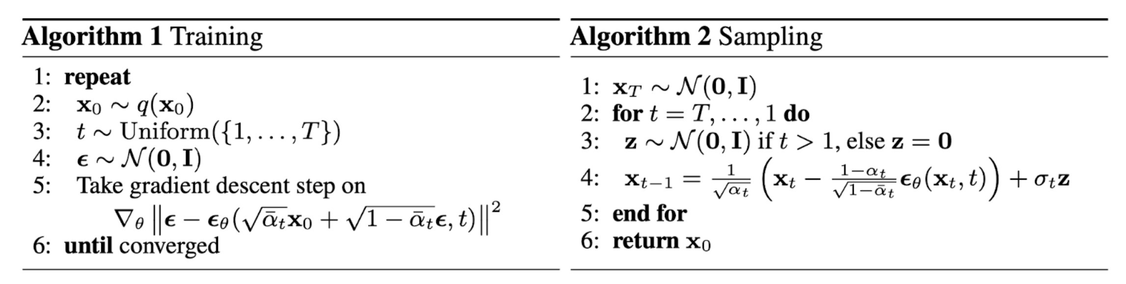
训练以及采样过程
现在对整体过程做一个总结:
训练时,对于某一时间步 t t t x t \mathbf{x}_t x t ϵ t \boldsymbol{\epsilon}_t ϵ t
推理采样时,从噪声出发,在 T T T x 0 \mathbf{x}_0 x 0
Reference